Statistics: Hypothesis Testing

Definitions

• Hypothesis Testing: A statistical method used to make decisions about a population parameter based on sample data. It involves evaluating two opposing hypotheses.

• Null Hypothesis (\(H_0\)): The statement being tested, representing no effect or no difference. It is the default assumption that there is no relationship between variables or no change from a specified value.

• Alternative Hypothesis (\(H_1\)): The statement that contradicts the null hypothesis, indicating the presence of an effect or a difference. It represents what we aim to prove.

Hypotheses

When conducting a hypothesis test, we start with an assumption (the null hypothesis) and then use sample data to assess whether there is enough evidence to reject this assumption in favor of an alternative hypothesis.

• Example: Suppose we want to test whether a new drug is effective in lowering blood pressure.

  • \(H_0\): The drug has no effect on blood pressure (i.e., the mean difference is zero).

  • \(H_1\): The drug lowers blood pressure (i.e., the mean difference is less than zero).

As in the example above, hypothesis testing is predicated on falsification, the idea that for a question or hypothesis to be scientific, it must be testable and able to be proven false.

When defining our hypotheses, the null hypothesis (\(H_0\)) represents the “status quo” or the idea that there is no effect, no difference, or no relationship between variables. In hypothesis testing, the null hypothesis is set up so that it can be rejected if evidence suggests otherwise, thus allowing researchers to assess the validity of the claim.

When we reject the null hypothesis, we often deem it to err toward the alternative hypothesis.

Note: Rejecting the null hypothesis does not prove the alternative hypothesis to be true. It merely suggests that the evidence is strong enough to conclude that the null hypothesis is unlikely given the data.

Notation

Null Hypothesis

\[ H_0: \theta = \theta_0 \]

Where

• \(\theta\) is the population parameter of interest.

• \(\theta_0\) is the hypothesized value of the population parameter under the null.

Note: Because the null hypothesis often represents the status quo, most null hypotheses we’ll encounter take the form of: \(H_0: \theta = 0\)

Alternative Hypothesis

\[\begin{split} H_1: \theta \begin{cases} > \theta_0 & \text{(Right-tailed)} \\ < \theta_0 & \text{(Left-tailed)} \\ \neq \theta_0 & \text{(Two-tailed)} \end{cases} \end{split}\]

Where the symbol of inequality is contingent on the type of hypothesis test (e.g., left, right, or two-tailed).

Procedure for Hypothesis Testing

1. Define Hypotheses (\(H_0\), \(H_1\))

The first step is to clearly state the null and alternative hypotheses. The null hypothesis typically reflects the status quo or a claim of no effect, while the alternative hypothesis reflects what we want to test.

2. Compute Test Statistic & Distribution

Once the hypotheses are defined, we calculate a test statistic based on the sample data. The test statistic quantifies how far the sample data deviates from the null hypothesis. Common test statistics include the \(z\)-score and \(t\)-statistic, depending on the sample size and whether the population standard deviation is known.

In general, test statistics are defined by:

\[ \text{Test Statistic} = \frac{\text{Point Estimate} - \text{Null Hypothesis}}{\text{Standard Error}} \]

or, more formally put:

\[ \text{Test Statistic} = \frac{\hat{\theta}-\theta_0}{SE(\hat{\theta})} \]

The distribution of the test statistic must be determined (e.g., normal distribution for large samples, \(t\)-distribution for small samples) to construct the test statistic.

• Example: For a sample mean test, the test statistic can be calculated as:

  \[ z = \frac{\bar{x} - \mu_0}{\frac{\sigma}{\sqrt{n}}} \sim \mathcal{N}(0,1) \]

  or, if population standard deviation is not known:

  \[ t = \frac{\bar{x} - \mu_0}{\frac{s}{\sqrt{n}}} \sim t_{n-1} \]

where \(\bar{x}\) is the sample mean, \(\mu_0\) is the population mean under \(H_0\), \(\sigma\) is the population standard deviation, \(s\) is the sample standard deviation, and \(n\) is the sample size.

3. Define Critical Region (\(\alpha\))

The critical region is the range of values for which we will reject the null hypothesis. It is determined by the significance level \(\alpha\), which represents the probability of making a Type I error (rejecting \(H_0\) when it is true). Common choices for \(\alpha\) are 0.05, 0.01, and 0.10.

The critical value(s) corresponding to \(\alpha\) can be found using the relevant distribution table (e.g., \(z\)-table, \(t\)-table).

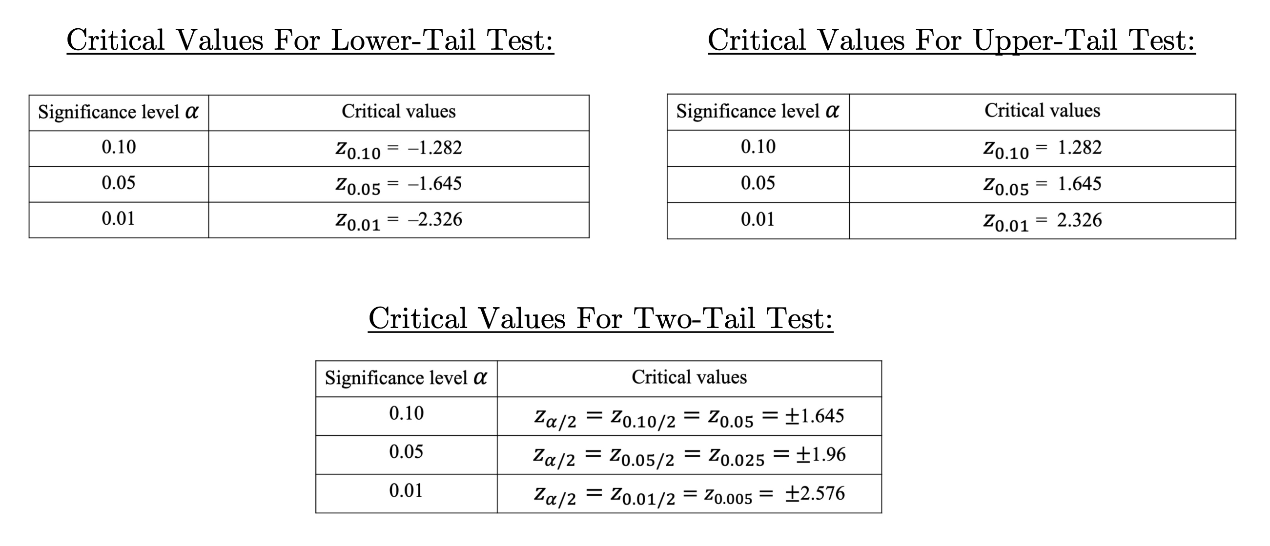
Critical Regions by Type of Test

Note: The critical region is determined by type of hypothesis test.

Recall:

\[\begin{split} H_1: \theta \begin{cases} > \theta_0 & \text{(Right-tailed)} \\ < \theta_0 & \text{(Left-tailed)} \\ \neq \theta_0 & \text{(Two-tailed)} \end{cases} \end{split}\]

For one-tailed tests (right/left), the critical region (\(\alpha\)) is the area above/below the critical value toward either sign of infinity. For two-tailed tests, the critical region is split in half (\(\alpha/2\)) on both tails above the two-tailed critical values.

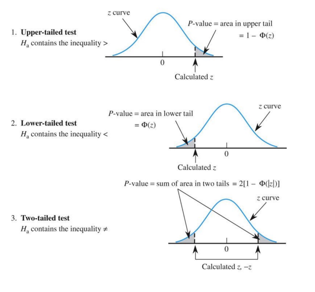
Image Source: https://link.springer.com/chapter/10.1007/978-1-4614-0391-3_9

4. Power of the Test

Statistical Power: The probability of correctly rejecting the null hypothesis when the alternative hypothesis is true. It reflects the test’s ability to detect an effect when there is one.

Formally, power (\(\kappa\)) is the probability of not committing a Type II error (failing to reject \(H_0\) when \(H_1\) is true):

\[ \kappa = 1-P(\text{Type II Error}) \]

Note: Formally, Type I and Type II errors are notated as \(\alpha\) and \(\beta\) respectively. Does seeing alpha ring a bell?

Our significance level (\(\alpha\)) is the Type I error rate. When we set our significance level, we are setting our acceptable Type I error rate. When we set our power, we are implicitly setting our accepted Type II error rate (\(1-\beta\)) where \(\beta\) is the Type II error rate.

Power is influenced by several factors:

• Sample Size (\(n\)): Larger samples generally lead to higher power because they provide more information about the population.

• Effect Size: The larger the true effect size (difference between the population parameter and null hypothesis), the higher the power.

• Significance Level (\(\alpha\)): Increasing \(\alpha\) increases the critical region, thereby increasing power, but also increases the risk of a Type I error.

A commonly accepted threshold for power is 0.80, meaning there is an 80% chance of correctly rejecting \(H_0\) when \(H_1\) is true.

5. Reject or Fail to Reject Null

After computing the test statistic, we compare it to the critical value(s):

• If the test statistic falls in the critical region, we reject \(H_0\).

• If the test statistic falls outside the critical region, we fail to reject \(H_0\).

In application, for a two-tailed test, this means that if \(|T|>|t^*|\) where \(t^*\) is the critical value, we reject the null hypothesis.

6. Draw Conclusions

The final step is to interpret the results in the context of the research question:

• If \(H_0\) is rejected, we conclude that there is sufficient evidence to support \(H_1\).

• If \(H_0\) is not rejected, we conclude that there is not enough evidence to support \(H_1\), but this does not prove that \(H_0\) is true.