Statistics: Estimation#
Definitions:#
Estimator: A rule or formula used to estimate an unknown population parameter based on sample data. For example, the sample mean \(\bar{x}\) is an estimator of the population mean \(\mu\).
Point Estimate: A single value estimate of a population parameter. For instance, \(\bar{x}\) is a point estimate for \(\mu\).
Standard Error (SE): The standard deviation of the sampling distribution of a statistic.
Point Estimation#
Estimator#
Recalling our discussion of estimators from the section on Populations & Samples, an estimator is a formula that defines our approach to estimating a population parameter \(\theta\). An estimator describes how to obtain a point estimate.
Point Estimate#
A point estimate is the realized value of an estimator \(\hat{\theta}\) given sample data. We can conceptualize it as our ‘best guess’ of \(\theta\)’s value.
Standard Error#
The standard error, simply put, is the standard deviation of some sample statistic. It measures the variability of an estimator \(\hat{\theta}\).
For the sample mean, for example:
where \(\sigma\) is the population standard deviation and \(n\) is the sample size.
Estimation Criteria#
When evaluating estimators, several important properties guide us in determining their quality:
Bias#
Bias refers to whether an estimator systematically overestimates or underestimates the true population parameter. An estimator is unbiased if its expected value equals the population parameter:
If \(E(\hat{\theta}) \neq \theta\), the estimator is biased. A biased estimator consistently misses the true value. We measure bias as the difference between \(E(\hat{\theta})\) and \(\theta\):
Bias of an Estimator#
Negatively Biased: \(\text{Bias}(\hat{\theta}) < 0\), “systematically underestimates \(\theta\) by…”
Unbiased: \(\text{Bias}(\hat{\theta}) = 0\), “precisely estimates \(\theta\)”
Positively Biased: \(\text{Bias}(\hat{\theta}) > 0\), “systematically overestimates \(\theta\) by…”
Note: Unbiasedness alone is not enough to determine the ‘best’ estimator.
Minimum Variance#
Among unbiased estimators, the best one is the one with the smallest variance, meaning it fluctuates less from sample to sample. The minimum variance criterion helps us choose estimators that are more reliable.
Given
We will choose \(\hat{\theta}_1\) over \(\hat{\theta}_2\) if
Efficient Estimator#
An estimator is considered efficient if it achieves the lowest possible variance among all unbiased estimators for a given parameter. This lowest possible variance is known as the Cramér-Rao Lower Bound (CRLB).
The CRLB sets a theoretical lower limit on the variance that any unbiased estimator of a parameter can achieve. If an estimator’s variance equals the CRLB, it is said to be efficient because it has the minimum possible variance for any unbiased estimator of that parameter.
Cramér-Rao Lower Bound (CRLB)#
The Cramér-Rao Lower Bound (CRLB) is given by:
Where:
\(\hat{\theta}\) is the estimator of the parameter \(\theta\),
\(\mathcal{I}(\theta)\) is the Fisher Information, a measure of how much information the data provides about the unknown parameter \(\theta\).
If an estimator’s variance equals \(\frac{1}{\mathcal{I}(\theta)}\), it is said to achieve the CRLB, meaning it is as “efficient” as possible.
Fisher Information#
The Fisher Information is calculated as:
Where \(L(\theta)\) is the likelihood function of the parameter \(\theta\), and the expectation is taken over the distribution of the observed data.
Efficient Estimator Example#
For instance, the sample mean \(\bar{X}\) of a normal distribution \(\mathcal{N}(\mu, \sigma^2)\) is an efficient estimator. The variance of the sample mean is:
The Fisher Information for this model is:
Thus, the CRLB is:
Since the variance of the sample mean equals the CRLB:
This shows that \(\bar{X}\) is an efficient estimator.
Proof that the Sample Mean Achieves the CRLB
Assume we have a sample \(X_1, X_2, \ldots, X_n\) drawn from a normal distribution \(\mathcal{N}(\mu, \sigma^2)\), where \(\mu\) is the unknown parameter we want to estimate, and \(\sigma^2\) is known.
Determine the Likelihood Function
The likelihood function \(L(\mu)\) for the normal distribution is given by:
\[ L(\mu) = \prod_{i=1}^{n} \frac{1}{\sqrt{2\pi\sigma^2}} \exp\left(-\frac{(X_i - \mu)^2}{2\sigma^2}\right)\]The log-likelihood function \(\ell(\mu)\) is:
\[ \ell(\mu) = \log L(\mu) = -\frac{n}{2} \log(2\pi\sigma^2) - \frac{1}{2\sigma^2} \sum_{i=1}^{n} (X_i - \mu)^2\]Calculate the First and Second Derivatives of the Log-Likelihood
First Derivative
The first derivative of the log-likelihood function with respect to \(\mu\) is:
\[ \frac{\partial \ell(\mu)}{\partial \mu} = \frac{1}{\sigma^2} \sum_{i=1}^{n} (X_i - \mu)\]Second Derivative
The second derivative is:
\[ \frac{\partial^2 \ell(\mu)}{\partial \mu^2} = -\frac{n}{\sigma^2}\]Compute the Fisher Information
The Fisher Information \(\mathcal{I}(\mu)\) is defined as the negative expected value of the second derivative of the log-likelihood:
\[ \mathcal{I}(\mu) = - \mathbb{E}\left[\frac{\partial^2 \ell(\mu)}{\partial \mu^2}\right] = -\left(-\frac{n}{\sigma^2}\right) = \frac{n}{\sigma^2}\]Cramér-Rao Lower Bound (CRLB)
The Cramér-Rao Lower Bound states:
\[\text{Var}(\hat{\mu}) \geq \frac{1}{\mathcal{I}(\mu)}\]Substituting the Fisher Information:
\[\text{Var}(\hat{\mu}) \geq \frac{\sigma^2}{n}\]Variance of the Sample Mean
Now, let’s calculate the variance of the sample mean \(\bar{X}\):
\[\bar{X} = \frac{1}{n} \sum_{i=1}^{n} X_i\]The variance of \(\bar{X}\) is:
\[\text{Var}(\bar{X}) = \text{Var}\left(\frac{1}{n} \sum_{i=1}^{n} X_i\right) = \frac{1}{n^2} \sum_{i=1}^{n} \text{Var}(X_i) = \frac{1}{n^2} \cdot n \sigma^2 = \frac{\sigma^2}{n}\]Compare Variance to CRLB
Since the variance of the sample mean \(\bar{X}\) equals the Cramér-Rao Lower Bound:
\[\text{Var}(\bar{X}) = \frac{\sigma^2}{n} = \frac{1}{\mathcal{I}(\mu)}\]This shows that the sample mean \(\bar{X}\) achieves the CRLB, confirming that it is an efficient estimator for the mean \(\mu\) of a normal distribution.
Note: For all intents and purposes, it is sufficient to understand efficiency of estimators to be the unbiased estimator \(\hat{\theta}^*\) with the lowest variance of all possible \(\hat{\theta}\).
Mean Squared Error (MSE)#
The mean squared error (MSE) combines both bias and variance to give an overall measure of an estimator’s accuracy:
An estimator with low MSE has both low bias and low variance, making it a reliable estimate of the population parameter.
Interval Estimation#
Confidence Intervals#
A confidence interval provides a range of values within which the population parameter is likely to fall, unlike point estimates that provide just a single value. The confidence interval is often expressed as:
For example, the confidence interval for the population mean \(\mu\) using the sample mean \(\bar{x}\) is:
where \(z_{\alpha/2}\) is the critical value from the standard normal distribution and \(\frac{\sigma}{\sqrt{n}}\) is the standard error of the sample mean.
Confidence Level#
The confidence level is the probability that the interval contains the true population parameter. Another way of conceptualizing confidence level is that it’s the probability that the true \(\theta\) falls within your confidence interval that you are okay with.
I.e., at a 95% CL, you are okay with the 5% chance that the true \(\theta\) takes a value outside of the specified range of values in your confidence interval. Or, intuitively, it’s saying:
“I’m 95% confident the population mean lies between these lower and upper limits.”
Common confidence levels are 90%, 95%, and 99%. A 95% confidence interval, for instance, means that if we took 100 different samples, approximately 95 of the intervals would contain the true parameter.
Significance Level (\(\alpha\))#
The significance level \(\alpha\) is the probability of rejecting a true population parameter. It is related to the confidence level by:
For a 95% confidence level, \(\alpha = 0.05\). This significance level determines the critical values and the rejection region in hypothesis testing.
Critical Region and Critical Value#
The critical region is the set of values that lead us to reject the null hypothesis (more on this in the next section). The critical value marks the boundary of this region and depends on the significance level. For a 95% confidence level, the critical value for a two-tailed standard normal distribution is \(z_{\alpha/2} = 1.96\).
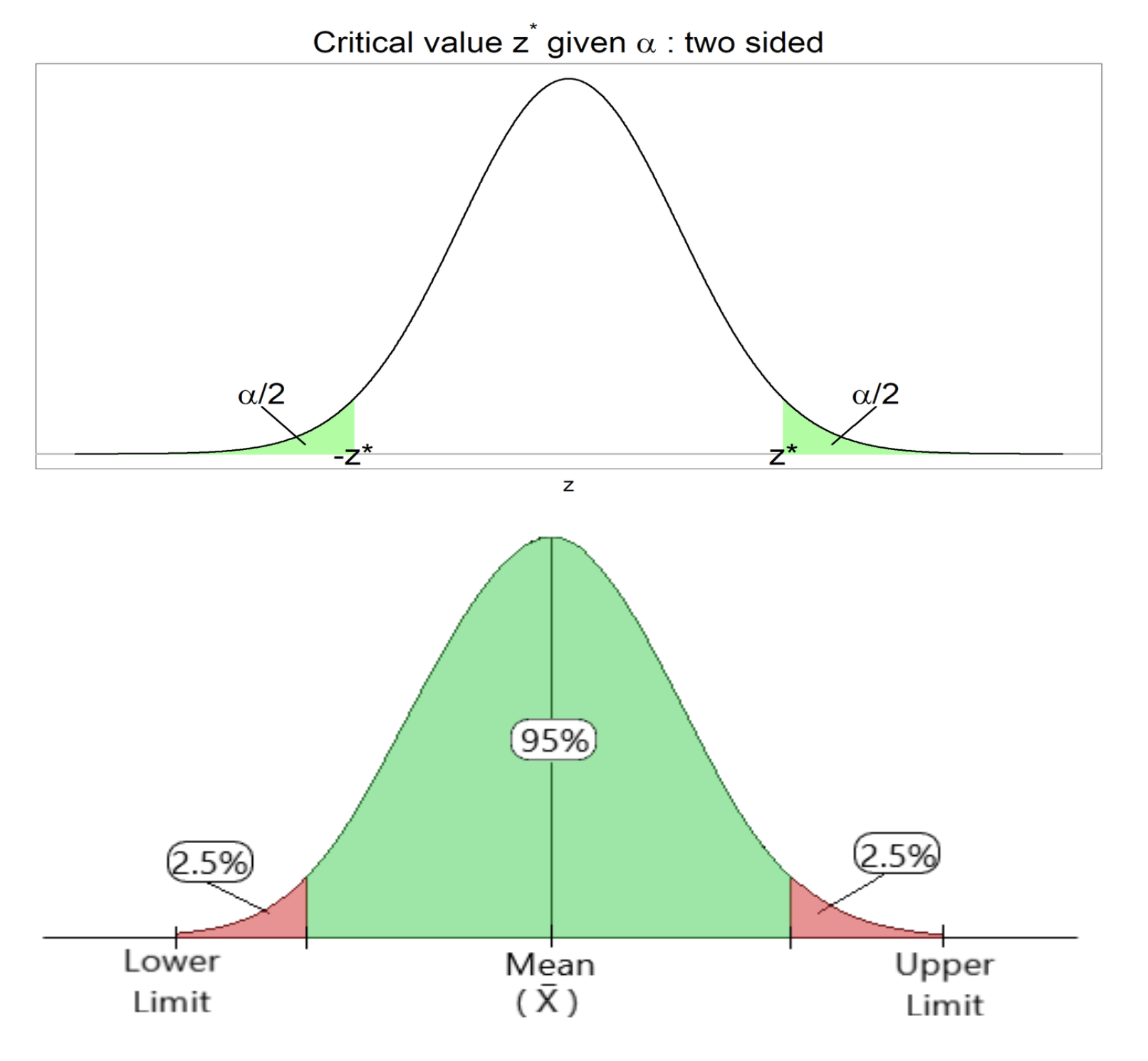
Image Source: https://statkat.com/find-critical-value/significance-level-alpha/t.php, https://memos.evergreencap.com/p/game-selection
Narrower Confidence Intervals: Smaller margin of error, thus more reliable estimate of \(\theta\)
Wider Confidence Intervals: Larger margin of error, thus less reliable estimate of \(\theta\)
Factors Determining the Width of the Confidence Interval#
Several factors influence the width of the confidence interval:
Level of Confidence: A higher confidence level results in a wider interval.
Variability: Greater variability in the data (larger \(\sigma\)) results in a wider interval.
Sample Size: Larger sample sizes result in narrower confidence intervals, as the standard error decreases with increased sample size.
Example: 90% Confidence Level, Two-Tail#
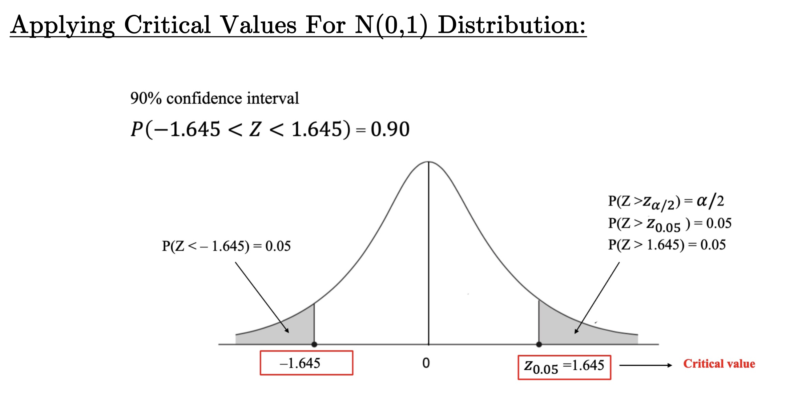
Image Source: PUBPOL 3100 Lecture Slides, Dr. Divya Deepthi
The \(t\)-Distribution#
The \(t\)-distribution is used instead of the normal distribution when the sample size is small or when the population standard deviation is unknown. It is similar to the normal distribution but has heavier tails, which account for the increased uncertainty.
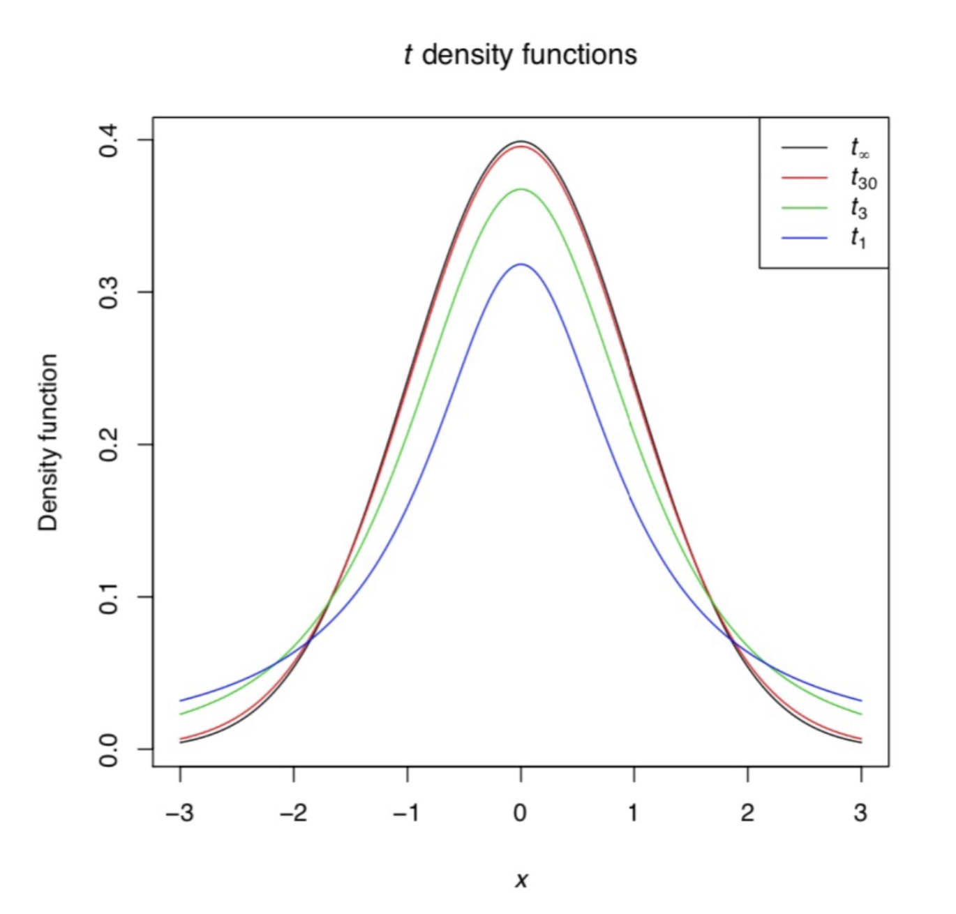
Image Source: PUBPOL 3100 Lecture Slides, Dr. Divya Deepthi
Note: In most (if not all) cases, the true population standard deviation is not known, meaning the \(t\)-distribution is the one we will use most.
Degrees of Freedom (\(df\))#
The shape of the \(t\)-distribution depends on the degrees of freedom (\(df\)), which is typically equal to \(n - 1\), where \(n\) is the sample size.
As \(n\) increases, the \(t\)-distribution approaches the normal distribution.
The Term “Degrees of Freedom:”
The concept of degrees of freedom arises from the idea that in a calculation, not all variables or parameters can vary freely. For instance, if you have a fixed sum (like the sample mean), knowing all but one of the values allows you to determine the last value. Thus, there is one less independent piece of information, indicating a restriction in the “freedom” of choice.
In statistics, then, the degrees of freedom typically represent the number of independent parameters that can be estimated.
Confidence Interval using \(t\)-Distribution#
When the population standard deviation \(\sigma\) is unknown, the confidence interval for the population mean \(\mu\) is calculated using the \(t\)-distribution:
where \(t_{\alpha/2, n-1}\) is the critical value from the \(t\)-distribution, \(s\) is the sample standard deviation, and \(n\) is the sample size.