Statistics: Probability

Definitions

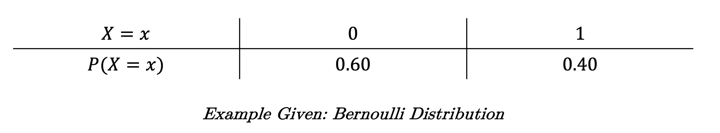
• Probability Distribution: A function that describes the likelihood of different outcomes for a random variable.

• Cumulative Distribution Function (CDF): A function that gives the probability that a random variable takes a value less than or equal to a certain threshold.

• Probability Density Function (PDF): A function that describes the likelihood of a continuous random variable taking on a specific value. The area under the PDF curve over an interval represents the probability that the random variable falls within that interval.

• Expected Value: The long-run weighted average outcome of repeated trials of a random variable.

• Variance: A measure of how much values of a random variable deviate from the expected value.

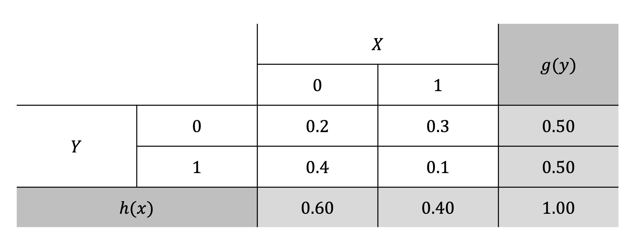
• Joint Probability Distribution: The probability distribution of two random variables considered together.

• Conditional Probability: The probability of one event occurring given that another event has already occurred.

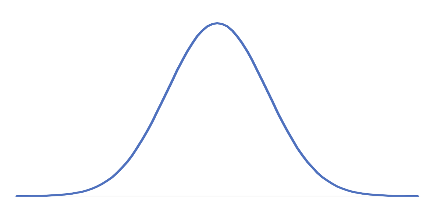
• Normal Distribution: A continuous probability distribution that is symmetric about its mean and forms a bell curve.

• Standard Normal Distribution: A special case of the normal distribution where the mean is 0 and the variance is 1.

• Z-Score: A standardized value that represents the number of standard deviations a data point is from the mean.

• Sampling Distribution: The probability distribution of a statistic (e.g., sample mean) based on repeated samples.

• Central Limit Theorem (CLT): The theorem stating that the distribution of the sample mean will approach a normal distribution as the sample size increases.

Probability

Probability deals with the likelihood of different outcomes occurring, particularly of random variables. When we try to understand probability, it’s helpful to think of repeated trials underpinning much of the theory; every time we repeat a trial, we can plot the outcome and construct distributions, or functions (that are often graphable!) that describe the likelihood of a particular outcome or value.

Probability Distributions

A probability distribution describes how the probabilities are distributed over the values of a random variable. There are two main types of probability distributions:

• Discrete Probability Distributions: These apply to random variables that take on a finite or countable number of possible values. The probability mass function (PMF) gives the probability that a discrete random variable is exactly equal to some value.

  • Example: The probability distribution of rolling a die, where the possible outcomes are 1 through 6, each with probability \(P(X = x) = \frac{1}{6}\).

• Continuous Probability Distributions: These apply to random variables that can take an infinite number of values. The probability density function (PDF) gives the likelihood of the variable taking a value within a particular range, as the probability of taking any specific value is technically 0.

  • Example: The normal distribution, which describes data that clusters around a mean in a bell-shaped curve.

Cumulative Probability Distributions

The cumulative distribution function (CDF) gives the probability that a random variable takes a value less than or equal to a certain threshold. For both discrete and continuous variables, it represents the accumulation of probabilities up to a given point.

• Formula (for discrete random variables):

  \[ F(x) = P(X \leq x) = \sum_{x_i \leq x} P(X = x_i) \]

• Formula (for continuous random variables):

  \[ F(x) = P(X \leq x) = \int_{-\infty}^{x} f(t) \, dt \]

  where \(f(t)\) is the probability density function (PDF).

Joint and Conditional Probability Distributions

• Joint Probability Distribution: The joint probability distribution of two random variables \(X\) and \(Y\) specifies the probability of different combinations of outcomes for \(X\) and \(Y\).

  \[ P(X, Y) \]

• Conditional Probability: The conditional probability of \(Y\) given \(X\) is the probability that \(Y\) occurs, given that \(X\) has already occurred:

  \[ P(Y| X = x) = \frac{P(X = x, Y = y)}{P(X = x)} \]

  Or, in other notation:

  \[ P(Y|X) = \frac{P(X \cap Y)}{P(X)} \]

Expected Value

Where the outcome of any particular trial produces a realized value, we often want to know the general expected value of a random variable. For example, it’s useful to know the expected recidivism rate from a pilot rehabilitation program that we can generalize from.

The expected value of a random variable is a measure of its central tendency, representing the long-term average outcome of repeated trials.

In other words, the expected value of a variable is equal to its mean, or the weighted average of all possible values, where the weights are the probabilities of each value occurring.:

\[ E(X) = \mu \]

• Formula (for discrete random variables): $\( E(X) = \sum_{i} x_i \cdot P(X = x_i) \)$

• Formula (for continuous random variables): $\( E(X) = \int_{-\infty}^{\infty} x \cdot f(x) \, dx \)$

Properties of Expected Value

1. Constant Rule: If \(a\) is constant, \(E(a) = a\)

2. Linearity of Expectation: If \(a\) and \(b\) are constants, \(E(aX + b) = a \cdot E(X) + b\)

3. Non-Linearity of Squaring: In general, \(E(X^2) \neq [E(X)]^2\)

4. Additivity of Expectations: If \(X\) and \(Y\) are random variables, \(E(X \pm Y) = E(X) \pm E(Y)\)

5. General Linearity of Expectation: If \(a\) and \(b\) are constants, \(E(aX \pm bY) = a \cdot E(X) \pm b \cdot E(Y)\)

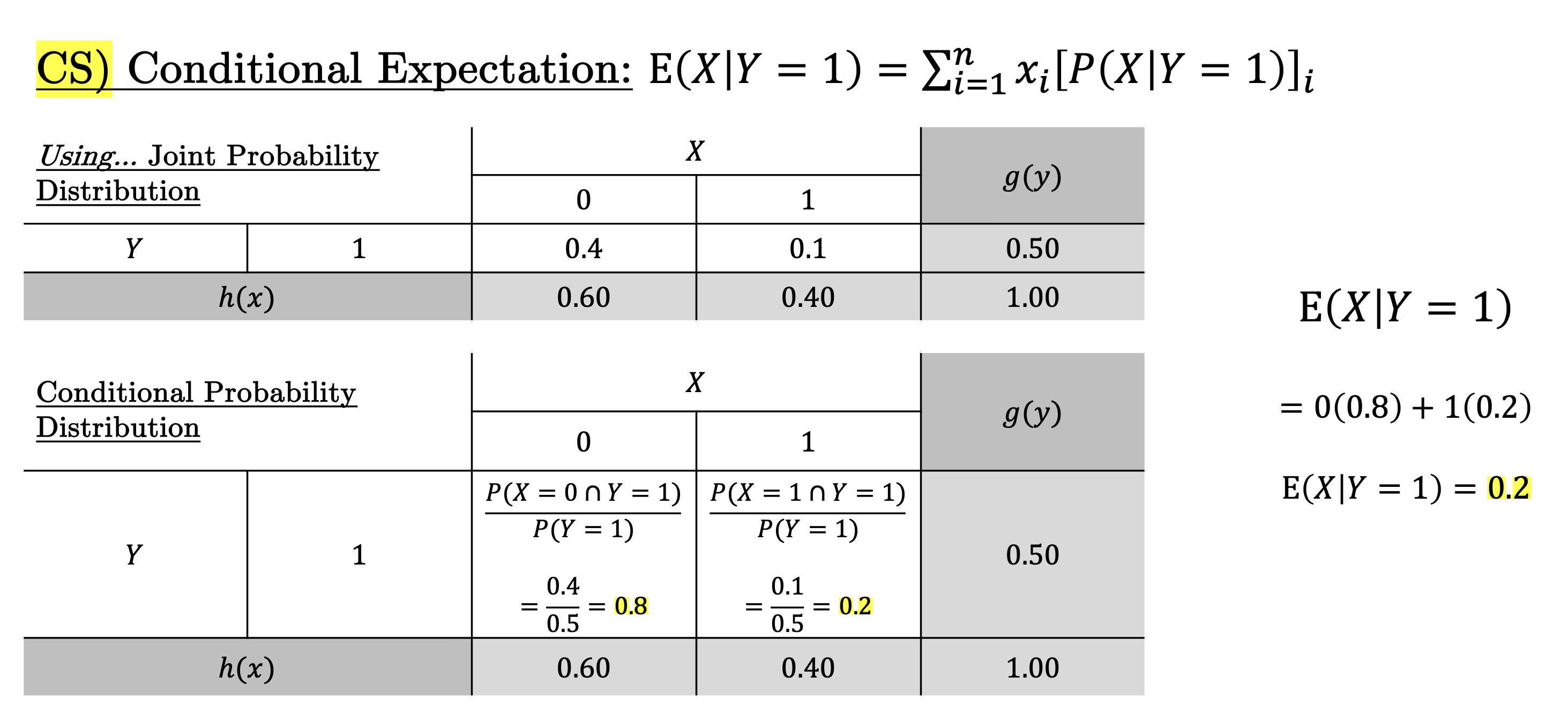
Conditional Expectation

In many situations, we’re interested in the expected value of a random variable, given that we have some additional information about another related variable. This is where conditional expectation comes into play.

The conditional expectation of a random variable \(X\), given another random variable \(Y\), represents the expected value of \(X\) when \(Y\) takes on a particular value. It helps us refine our predictions for \(X\) based on knowledge of \(Y\).

Formula (for discrete random variables):

\[ E(X \mid Y = y) = \sum_{i} x_i \cdot P(X = x_i \mid Y = y) \]

Formula (for continuous random variables):

\[ E(X \mid Y = y) = \int_{-\infty}^{\infty} x \cdot f_{X|Y}(x \mid y) \, dx \]

Here, \(f_{X|Y}(x \mid y)\) represents the conditional probability density function of \(X\) given \(Y = y\).

Conditional expectation allows us to focus on a subset of data or scenarios by adjusting our expectation based on known information. For instance, if we want to know the expected sales in a store, given that there was heavy rainfall, the conditional expectation lets us calculate that adjusted expectation using only data where the condition (rainfall) holds.

Example

Law of Iterated Expectations

In general, the relationship between conditional expectation and standard expectation can be written as:

\[ E(X) = E\left[E(X \mid Y)\right] \]

This equation reflects that the overall expected value of \(X\) can be broken down into the weighted average of its conditional expectations across all possible values of \(Y\). This is known as the Law of Iterated Expectations. This property is particularly useful in probability theory and statistics for breaking complex expectations into simpler components.

Variance

While the expected value gives us an idea of the central tendency, variance measures the spread or dispersion of a random variable around its mean. Specifically, variance quantifies how much the values of a random variable differ from the expected value.

Variance is particularly useful when comparing the consistency of different random variables or when understanding the variability within the same variable across different contexts.

The variance of a random variable is defined as the expected value of the squared deviations from its mean:

\[\begin{split} \begin{align*} \text{Var}(X) &= E\left[(X - \mu)^2\right] \\ &= E(X^2) - [E(X)]^2 \end{align*} \end{split}\]

• Formula (for discrete random variables): $\( \text{Var}(X) = \sum_{i} P(X = x_i) \cdot (x_i - \mu)^2 \)$

• Formula (for continuous random variables): $\( \text{Var}(X) = \int_{-\infty}^{\infty} (x - \mu)^2 \cdot f(x) \, dx \)$

Properties of Variance

1. Variance of a Constant: If \(a\) is constant, \(\text{Var}(a) = 0\)

2. Scaling Rule: If \(a\) is constant, \(\text{Var}(aX) = a^2 \cdot \text{Var}(X)\)

3. Variance of a Linear Transformation: If \(a\) and \(b\) are constants, \(\text{Var}(aX + b) = a^2 \cdot \text{Var}(X) + 0\)

4. Additivity of Variance of Independent Variables: If \(X\) and \(Y\) are independent random variables, \(\text{Var}(X + Y) = \text{Var}(X) + \text{Var}(Y)\)

5. Difference of Independent Variables: If \(X\) and \(Y\) are independent random variables, \(\text{Var}(X - Y) = \text{Var}(X) + \text{Var}(Y)\)

Normal Distribution

The normal distribution is a continuous probability distribution that is symmetric about its mean and follows the shape of a bell curve. It is one of the most important distributions in statistics because of its frequent occurrence in natural and social phenomena.

• Probability density function (PDF) of the normal distribution:

  \[ f(x) = \frac{1}{\sigma \sqrt{2\pi}} \exp \left( -\frac{(x - \mu)^2}{2\sigma^2} \right) \]

  where \(\mu\) is the mean and \(\sigma^2\) is the variance.

• Cumulative distribution function (CDF) of the normal distribution:

  \[ F(x) = P(X \leq x) = \int_{-\infty}^{x} \frac{1}{\sigma \sqrt{2\pi}} \exp \left( -\frac{(t - \mu)^2}{2\sigma^2} \right) dt \]

Probability Density Function (PDF)

\[ f(x) = \frac{1}{\sigma \sqrt{2\pi}} \exp \left( -\frac{(x - \mu)^2}{2\sigma^2} \right) \]

The PDF describes the likelihood of a continuous random variable \(X\) taking on a specific value \(x\).

Parameters:

• \(\mu\): The mean of the distribution, which represents the center of the distribution.

• \(\sigma\): The standard deviation, which measures the spread of the distribution around the mean.

Explanation:

The term \(\frac{1}{\sigma \sqrt{2\pi}}\) is a normalization constant that ensures the total area under the PDF curve equals 1, which is a requirement for all probability density functions.

The expression \(\exp \left( -\frac{(x - \mu)^2}{2\sigma^2} \right)\) gives the exponential decay of the probability density as you move away from the mean. The PDF is symmetric about the mean, and its shape is determined by the standard deviation; a smaller \(\sigma\) leads to a steeper curve, while a larger \(\sigma\) results in a flatter curve.

Cumulative Distribution Function (CDF)

\[ F(x) = P(X \leq x) = \int_{-\infty}^{x} \frac{1}{\sigma \sqrt{2\pi}} \exp \left( -\frac{(t - \mu)^2}{2\sigma^2} \right) dt \]

The CDF provides the probability that a random variable \(X\) will take on a value less than or equal to \(x\). In other words, it accumulates the probabilities from the left tail of the distribution up to the point \(x\).

Explanation:

The CDF is calculated by integrating the PDF from \(-\infty\) to \(x\). This integral sums all the infinitesimally small probabilities (densities) from the left end of the distribution up to the specified value \(x\).

The result of the integral, \(F(x)\), gives a value between 0 and 1, which represents the probability of observing a value less than or equal to \(x\).

The CDF is a non-decreasing function, meaning it will never decrease as \(x\) increases. As \(x\) approaches \(-\infty\), \(F(x)\) approaches 0, and as \(x\) approaches \(+\infty\), \(F(x)\) approaches 1.

Note: It is most likely the case that you will never need to know the formulas for the PDF or CDF. Nonetheless, they are provided and explained in the rare chance you need them for reference.

Standardization and Z-Scores

Standardization refers to the process of transforming a random variable \(X\) with mean \(\mu\) and standard deviation \(\sigma\) into a standard normal variable \(Z\), which has mean 0 and variance 1: $\( Z = \frac{X - \mu}{\sigma} \)$ This transformation allows comparison across different distributions and forms the basis for hypothesis testing and confidence intervals (see next section).

It cannot be understated:

Standardization allows us to compare variables across different units.

This is instrumental in allowing us to compare apples to apples and make meaningful inferences.

Standard Normal Distribution

The standard normal distribution is a special case of the normal distribution where the mean \(\mu = 0\) and the variance \(\sigma^2 = 1\).

• Z-Score: Any normal random variable \(X\) can be transformed into the standard normal distribution using a Z-score:

  \[ Z = \frac{X - \mu}{\sigma} \]

  Where \(Z=z\) is the standardized z-score for every \(X=x\). This allows comparison of different normal distributions on the same scale.

• Standard Normal CDF: The CDF of the standard normal distribution is denoted as \(\Phi(z)\), or the area under the curve up to a particular z-score.

Sampling Distributions

A sampling distribution is the probability distribution of a statistic (like the sample mean or variance) based on a random sample. The sampling distribution describes how the statistic varies from sample to sample.

Key Statistic: The sample mean \(\bar{X}\) has its own distribution, especially important for large samples under the Central Limit Theorem (CLT).

Central Limit Theorem (CLT)

The Central Limit Theorem (CLT) states that, given a sufficiently large sample size, the sampling distribution of the sample mean \(\bar{X}\) will be approximately normal, regardless of the distribution of the population from which the sample is drawn.

\[ \bar{X} \sim N\left(\mu, \frac{\sigma^2}{n}\right) \]

This approximation improves as the sample size \(n\) increases.

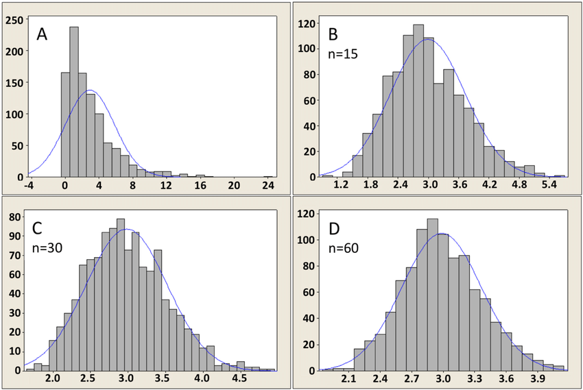
Image Source: https://mathematicalmysteries.org/central-limit-theorem/

The CLT is foundational in inferential statistics because it allows us to make probability statements about sample means even when the population distribution is unknown.

In general, CLT applies when \(n\geq 30\) at minimum. But, the actual minimum size can depend on the characteristics of the population distribution and the specific context of the analysis. For populations that are heavily skewed or have outliers, larger samples may be required to ensure the sampling distribution of the mean is approximately normal.

Note: We will return to how to calculate sample size later in the Causal Inference section on power.

Overview of Probability Distributions

1. Bernoulli Distribution:

   • Represents a single trial with two possible outcomes: success (\(1\)) and failure (\(0\)).

   • Probability Mass Function (PMF):

     \[ P(X = x) = p^x (1 - p)^{1 - x} \quad \text{for } x = 0, 1 \]

   • Parameter: \(p\) (probability of success).

2. Binomial Distribution:

   • Describes the number of successes in \(n\) independent Bernoulli trials.

   • PMF:

     \[ P(X = k) = \binom{n}{k} p^k (1 - p)^{n - k} \]

     where \(k = 0, 1, \dots, n\).

   • Parameters: \(n\) (number of trials), \(p\) (probability of success).

3. Geometric Distribution:

   • Models the number of trials until the first success in a series of Bernoulli trials.

   • PMF:

     \[ P(X = k) = (1 - p)^{k - 1} p \]

     where \(k = 1, 2, 3, \dots\).

   • Parameter: \(p\) (probability of success).

4. Poisson Distribution:

   • Represents the number of events occurring in a fixed interval, assuming the events happen independently.

   • PMF:

     \[ P(X = k) = \frac{\lambda^k e^{-\lambda}}{k!} \]

     where \(k = 0, 1, 2, \dots\).

   • Parameter: \(\lambda\) (average rate of occurrence).

5. Exponential Distribution:

   • Models the time between events in a Poisson process.

   • PDF:

     \[ f(x) = \lambda e^{-\lambda x} \quad \text{for } x \geq 0 \]

   • Parameter: \(\lambda\) (rate of occurrence).

6. Uniform Distribution:

   • All outcomes are equally likely within a defined range.

   • PDF (continuous):

     \[ f(x) = \frac{1}{b - a} \quad \text{for } a \leq x \leq b \]

   • Parameters: \(a\) (minimum), \(b\) (maximum).

7. Chi-Squared Distribution:

   • A distribution of the sum of squares of \(k\) independent standard normal random variables.

   • PDF:

     \[ f(x; k) = \frac{1}{2^{k/2} \Gamma(k/2)} x^{k/2 - 1} e^{-x/2} \quad \text{for } x > 0 \]

   • Parameter: \(k\) (degrees of freedom).